zernpol documentation
This simple package offers tools to handle Zernike Polynoms and the different indexing systems (as the Noll system for instance).
The package offers object and non-object oriented functions.
Install
From pip:
> pip install zernpol
From sources:
> git clone https://gricad-gitlab.univ-grenoble-alpes.fr/guieus/zernpol.git
> cd zernpol
> python setup.py install
Usage
zernpol
The zernpol.zernpol() function is almost all whats one needs.
It creates one or a list of zernpol.Zernpol object which is basically a 2 tuple
with some useful properties and methods from various input parameters.
In the following all examples are equivalents:
>>> from zernpol import zernpol, Zernpol
>>> zernpol( (2,-2) )
Zernpol(2, -2)
>>> Zernpol(2,-2)
Zernpol(2, -2)
>>> z = zernpol(5) # 5 is the index number system here in the default Noll system
Zernpol(2, -2)
>>> z = zernpol(5, 'Noll')
Zernpol(2, -2)
>>> z = zernpol(3, 'Ansi')
Zernpol(2, -2)
>>> z = Zernpol.from_noll(5)
Zernpol(2, -2)
>>> z = zernpol('astig_0')
Zernpol(2, -2)
The zernpol.zernpol() function accept also iterable, as list for instance, and will return a list of
zernpol.Zernpol :
>>> from zernpol import zernpol
>>> [z.name for z in zernpol( range(1,10) )] # default is Noll index  system
['piston',
 'tip',
 'tilt',
 'defocus',
 'astig_0',
 'astig_45',
 'comax',
 'comay',
 'trifoll_0']
Indexing system
The used system can be change from a string or thanks to the zernpol.ZIS (for Zernike Indexing system)
containing functions to convert back and forward zernike polynom coefficients to indexes or indexes to
zernike polynom coefficients
>>> from zernpol import zernpol, ZIS
>>> zernpol( range(1,5), ZIS.Noll)
[Zernpol(0, 0), Zernpol(1, 1), Zernpol(1, -1), Zernpol(2, 0)]
>>> zernpol( range(1,5), ZIS.Ansi) # zernpol( range(1,5), 'Ansi') also works
[Zernpol(1, -1), Zernpol(1, 1), Zernpol(2, -2), Zernpol(2, 0)]
Four Indexing systems exists (defined on wikipedia):
These classes can also be simply used to convert index to zernike polynoms or the contrary
>>> from zernpol import ZIS
>>> ZIS.Noll.i2z(5)
Zernpol(2, -2)
>>> ZIS.Noll.z2i((2,-2))
5
The default indexing system, used when the second optional argument of zernpol.zernpol() is None,
is contained inside the zernpol.ZIS as zernpol.ZIS.Default parameters. One can change
it with cautions at the highest level of an application:
>>> from zernpol import ZIS, zernpol
>>> ZIS.Default = ZIS.Ansi
>>> zernpol(3)
Zernpol(2, -2)
>>> ZIS.Default = ZIS.Noll
>>> zernpol(3)
Zernpol(1, -1)
Build the polynom
The zernpol.Zernpol.func() and zernpol.Zernpol.func_cart() are used to build the zernike polynomials from
polar and cartesian coordinate respectively.
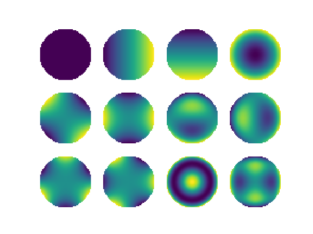
>>> from zernpol import zernrange, zernpol_func_cart
>>> from matplotlib.pylab import plt
>>> import numpy as np

>>> X,Y = np.meshgrid( np.linspace(-1,1,50), np.linspace(-1,1,50))
>>> fig, axs = plt.subplots(3,4)
>>> for zp,ax in zip(zernrange(1,13),axs.flat):
>>>    ax.imshow(zp.func_cart(X,Y))
>>>    ax.axis('off')
The zernpol.zernpol_func() and zernpol.zernpol_func_cart() function do the same but in a vectorialised
fashion optimised for array of zernike polynome coefficients
>>> from zernpol import zernpol, zernpol_func_cart
>>> import numpy as np

>>> X,Y = np.meshgrid( np.linspace(-1,1,50), np.linspace(-1,1,50))
>>> Z = zernpol_func_cart( zernpol(range(1,13)), X, Y)
>>> Z.shape
(12, 50, 50)
>>> from zernpol import zernpol_func, zernrange
>>> import numpy as np
>>> from matplotlib.pylab import plt
>>> r,theta = np.linspace(0,1,50), np.pi/4.
>>> plt.plot(r,  zernpol_func( zernrange(1,21), r,theta).T )
>>> plt.gca().set( title="20 first zernike modes at pi/4", xlabel="r")
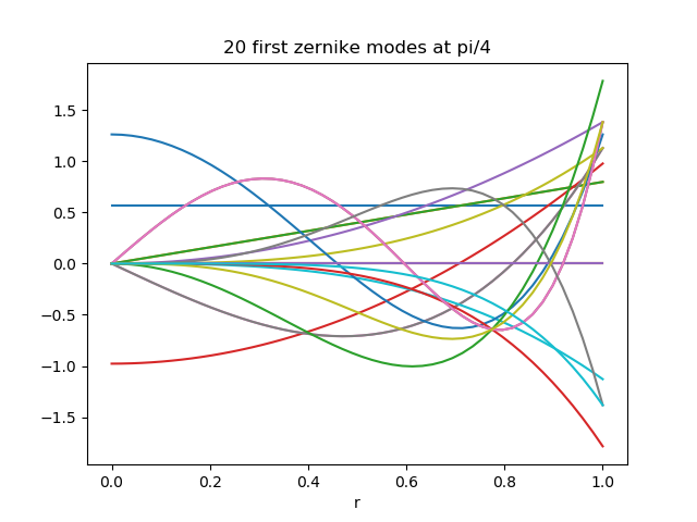
Note
On the example above zernrange(1,21) is similar to zernpol(range(1,21))
By default the zernike polynoms are normalised to rms = 1
>>> from zernpol import zernpol, zernpol_func_cart
>>> import numpy as np

>>> X,Y = np.meshgrid( np.linspace(-1,1,2000), np.linspace(-1,1,2000))
>>> Z = zernpol_func_cart( zernpol(range(1,13)), X, Y)
>>> rms = np.sqrt( np.nanmean(Z**2, axis=(1,2)) )
>>> rms
array([1.        , 0.99998983, 0.99998983, 0.99997967, 1.00002123,
   0.99993809, 0.99996952, 0.99996952, 0.9999695 , 0.9999695 ,
   0.99995938, 0.99989017])
Pupil
For wavefront analysis one have to project the zernike polynomes over a specific portion of an 2d
image. For this zernpol provides two things the zernpol.zernpol_pupil() (and its zernpol.Zernpol.func_pupil() homolog)
function and the zernpol.PupilMask.
zernpol.zernpol_pupil() is using zernpol.PupilMask to project the zernike polynomes in
an image. zernpol.PupilMask has several parameters:
zernpol.PupilMask.maskthe 2d boolean mask where True determine illuminated phase screen pixels
zernpol.PupilMask.radiusis the true radius (in fraction of pixel) of the the pupil where zernike polynoms will be projected
zernpol.PupilMask.centertrue (x0,y0) coordinates of the pupil center
zernpol.PupilMask.angle(default 0.0) the angle of projection of zernike polynomials
zernpol.PupilMask.flip2 tuple of 1 or -1 to determine any flip in the zernike polynoms for instance (-1,1) if a flip in x direction only, (1,1) is no flip at all.
They are several ways to create a zernpol.PupilMask and probably one will want to custom function
to application (for instance from an Influence Function matrix).
However zernpol offer basic ways :
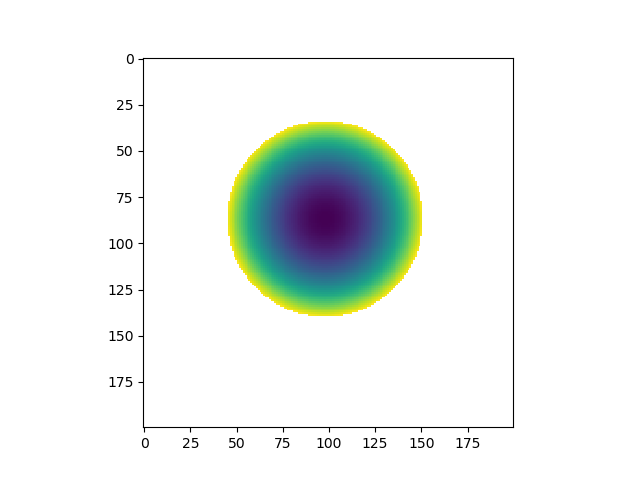
>>> from zernpol import PupilDisk, zernpol
>>> from matplotlib.pylab  import plt
>>> disk = PupilDisk(36.0) # A disk with a 36mm radius (the unit does not mater, see below)
>>> mask = disk.make_mask( [200,200], scale=0.34, center=[98,87] ) # scale is in User Unit/pixel
>>> plt.imshow(zernpol(4).func_pupil( mask ))
>>> plt.show()
The zernpol.func_pupil() is the vectorialized alternative :
>>> from zernpol import PupilDisk, zernpol, zernpol_pupil
>>> mask = PupilDisk(36.0).make_mask( [200,200], scale=0.34, center=[98,87] )
>>> zernpol_pupil( list(zernrange(1,15)), mask ).shape
(14, 200, 200)
The array returned can have a lot of NaN values when the image is large and the illuminated spot is small. The inpupil_only keyword allows to return only phases of illuminated pixel in a flat vector (per zernikes). This allow to reduce the memory footprint of a matrix of zernike polynoms and reduce computation time when multiplying or inverting matrix.
Following the last example:
>>> zernikes = zernpol_pupil( list(zernrange(1,15)), mask, inpupil_only=True )
>>> zernikes.shape
(14, 8789)
One can however reconstruct the images easily with the zernpol.PupilMask.reconstruct() method
>>>  mask.reconstruct(zernikes).shape
(14, 200, 200)
The simple reverse operation can be done easily as well (to remove NaN of a mesured phase screen for instance).
>>> mask.deconstruct(  mask.reconstruct(zernikes) ).shape
(14, 8789)
A zernpol.PupilMask can be build with zernpol.mask_from_image() and from a 2d image
where guess of the projected zernike mode radius is made from the illuminated mask of the pupil and
the its center from the baricenter of illuminated pixels.
>>> import numpy as np
>>> from zernpol import mask_from_image
>>> x,y = np.meshgrid( np.arange(200), np.arange(200))
>>> z = np.random.random( (200,200) )
>>> z[ np.sqrt( (x-98.2)**2+(y-87.6)**2 )>52.3 ] = np.nan
>>> mask = mask_from_image(z)
>>> mask.radius, mask.center
(51.75, (98.18354283054003, 87.58088919925513))
As seen above the pixel digitalisation will make the radius and center accurate at ~1/2 pixel
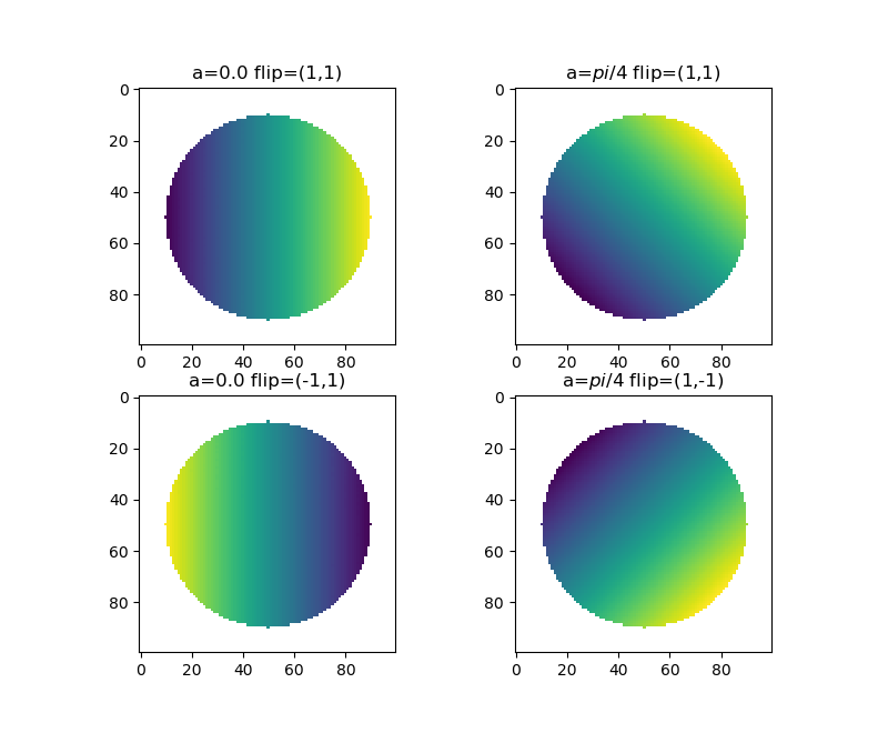
The example bellow demonstrate the effect of the flip and the angle parameters:
>>> from zernpol import PupilDisk, zernpol
>>> from matplotlib.pylab  import plt
>>> import numpy as np
>>> disk = PupilDisk(80)

>>> ax = plt.subplot(221)
>>> plt.imshow( zernpol(2).func_pupil( disk.make_mask([100,100], angle=0.0, flip=(1,1) )))
>>> ax.set_title("a=0.0 flip=(1,1)")

>>> ax = plt.subplot(222)
>>> plt.imshow( zernpol(2).func_pupil( disk.make_mask([100,100], angle=np.pi/4, flip=(1,1) )))
>>> ax.set_title("a=$pi/4$ flip=(1,1)")

>>> ax = plt.subplot(223)
>>> plt.imshow( zernpol(2).func_pupil( disk.make_mask([100,100], angle=0.0, flip=(-1,1) )))
>>> ax.set_title("a=0.0 flip=(-1,1)")

>>> ax = plt.subplot(224)
>>> plt.imshow( zernpol(2).func_pupil( disk.make_mask([100,100], angle=np.pi/4, flip=(1,-1) )))
>>> ax.set_title("a=$pi/4$ flip=(1,-1)")
>>> plt.show()
Misc features
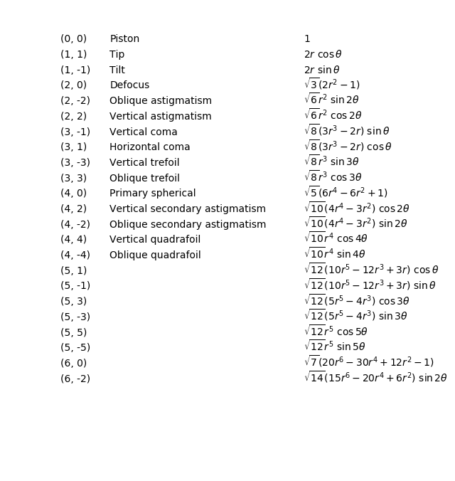
A latex equation representing the zernike polynomial can be reached :
>>> from zernpol import zernpol
>>> z = zernpol(5)
>>> z.latex
'\\sqrt{6} r^{2} \\ \\sin{\\,2\\theta}'
Is equivalent to:
>>> from zernpol import latex_formula
>>> latex_formula((2, -2))
'\\sqrt{6} r^{2} \\ \\sin{\\,2\\theta}'
>>> from zernpol import zernpol
>>> from matplotlib.pylab import plt
>>> for i,z in enumerate(zernpol(range(1,24))):
>>>     y = 24-i
>>>     plt.text(0.7 ,y, "$"+z.latex+"$")
>>>     plt.text(0.15,y, z.long_name)
>>>     plt.text(0.01,y, z)
>>> plt.gca().set( ylim=(-1, i+1))
>>> plt.gca().axis('off')
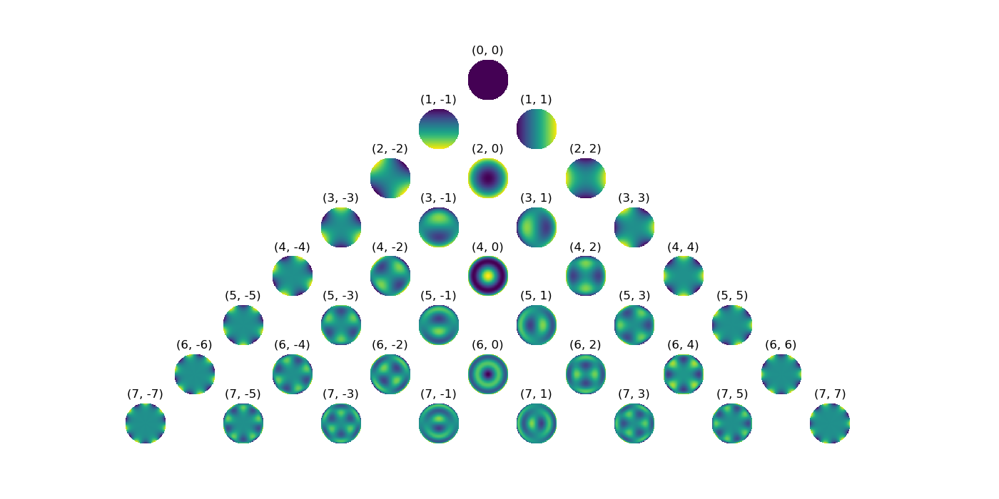
for the fun of it, a pyramide of zernike polynoms
>>> from zernpol import zernpol_func_cart
>>> from matplotlib.pylab import plt
>>> x,y = np.meshgrid(np.linspace(-1,1,100), np.linspace(-1,1,100))
>>> ns = range(0,8)
>>> f,axs = plt.subplots(8,16)
>>> for a in axs.flat: a.axis('off')
>>> for n in ns:
>>>     for m in range(-n,n+1,2):
>>>         axs[n, 7+m].imshow( zernpol_func_cart((n,m),x,y) )
>>>         axs[n, 7+m].set_title((n,m))
>>> plt.gcf().set_size_inches( 14, 7 )
Module Indexes
See also Alphabetical Index
- class zernpol.ZIS
A set of zernike polynomial indexing system
- class Ansi
Define the zernike polynomials OSA/ANSI indexing system
see: https://en.wikipedia.org/wiki/Zernike_polynomials#OSA/ANSI_standard_indices
- Arizona
alias of
zernpol._zernpol.Fringe
- Default
alias of
zernpol._zernpol.Noll
- class Fringe
Define the zernike polynomials Fringe/University of Arizona indexing system
see: https://en.wikipedia.org/wiki/Zernike_polynomials#Fringe/University_of_Arizona_indices
- static i2z(j)
convert Fringe/University of Arizona indice to zernike polynoms
- class Noll
Define the zernike polynomials Noll indexing system
see:
- static i2z(j: int) Tuple[int, int]
convert noll indice to zernike polynom coefficients
see https://en.wikipedia.org/wiki/Zernike_polynomials#Noll’s_sequential_indices
- Osa
alias of
zernpol._zernpol.Ansi
- class Wyant
Define the zernike polynomials Wyant indexing system
see: https://en.wikipedia.org/wiki/Zernike_polynomials#https://en.wikipedia.org/wiki/Zernike_polynomials#Wyant_indices
- static i2z(j)
convert Wyant indice to zernike polynomials (n,m)
- ansi
alias of
zernpol._zernpol.Ansi
- fringe
alias of
zernpol._zernpol.Fringe
- noll
alias of
zernpol._zernpol.Noll
- osa
alias of
zernpol._zernpol.Ansi
- wyant
alias of
zernpol._zernpol.Wyant
- class zernpol.Zernpol(n, m)
Usefull class holding zernike polynoms coefficient
a Zernpol can also be build from Zernpol.from_* functions where * is the name of the indexing system
>>> Zernpol.from_noll(3) == Zernpol.from_ansi(1)
True
>>> Zernpol.from_name('tilt')
Zernpol(1, -1)
- Parameters
n – Zernike polynom coefficients
m – Zernike polynom coefficients
- func_pol()
zernike polynom from polar coordinates
- func_cart()
zernike polynom from cartezian coordinates
- name, long_name
name and long name ( up to ‘quadrafoil_0’ noll=15)
- Type
Example:
>>> from zernpol import Zernpol, zernpol
>>> import numpy as np
>>> z = Zernpol(2,-2)
>>> z.name, z.long_name
('astig_0', 'Oblique astigmatism')
>>> x,y = np.meshgrid( np.linspace(-1,1,50) , np.linspace(-1,1,50) )
>>> phase_screen = z.func_cart(x,y)
- property ansi
OSA/Ansi index
- property fringe
Fringe/ University of Arizona index
- func(r, theta, normalized=True, masked=True)
Zernike Polynomial function from native polar coordinates
If you look for the vectorialized counterpart function see
zernpol_func()- Parameters
r (float, array) – radial and polar value. r and theta shall be broadcast together
theta (float, array) – radial and polar value. r and theta shall be broadcast together
normalized (boolean, optional) – if True (default), the polynom is normalized to 1
masked (boolean, optional) – if True all values outside the r=1 (above r>) is masked by nan values
- Ouputs:
z: float of array with shape r.shape
Example:
>>> import numpy as np
>>> from zernpol import zernpol
>>> r, theta = np.meshgrid( np.linspace(0, 1, 50), np.linspace(0, 2*np.pi, 50) )
>>> z4 = zernpol(4)
>>> z4.func(r, theta).shape
(50, 50)
Plot astig for several theta
>>> import numpy as np
>>> from matplotlib.pylab import plt
>>> from zernpol import zernpol
>>> r, theta = np.meshgrid( np.linspace(0, 1, 50), [0, np.pi/8, np.pi/4] )
>>> zp = zernpol('astig_0')
>>> a = zp.func(r, theta)
>>> [plt.plot(r[0], z) for z in a]
- func_cart(x, y, normalized=True, masked=True)
Zernike Polynomial function cartezian coordinates
If you look for the vectorialized counterpart function see
zernpol_func_cart()- Parameters
x (float, array) – x and y coordinate of phase screen. x and y shall be broadcast together
y (float, array) – x and y coordinate of phase screen. x and y shall be broadcast together
normalized (boolean, optional) – if True (default), the polynom is normalized to 1
masked (boolean, optional) – if True all values outside the $r^2= x^2+y^2=1$ is masked by nan values
- Returns
float of array with shape x.shape
- Return type
z
Example:
>>> import numpy as np
>>> from matplotlib.pylab import plt
>>> from zernpol import zernpol
>>> x, y = np.meshgrid( np.linspace(-1, 1, 50), np.linspace(-1, 1, 50) )
>>> nm = zernpol( range(1,10) )
>>> z4 = zernpol(4)
>>> plt.imshow( z4.func_cart(x,y) )
- property info
All information inside a dictionary
- property latex
LaTeX Formula
- property noll
Noll index
- property wyant
Wyant index
- zernpol.ansi_to_zernpol(j)
convert OSA/ANSI indice to zernike polynoms
- zernpol.fringe_to_zernpol(j)
convert Fringe/University of Arizona indice to zernike polynoms
- zernpol.latex_formula(nm: Tuple[int, int])
Return the latex formula of zernike polynom
- Parameters
nm (tuple,
Zernpol) – zernike n,m polynom coeeficients- Returns
LaTex Formula
- Return type
formula (str)
Note
The return formula is not bracketed by ‘$’
Example:
>>> from zernpol import latex_formula, Zernpol, zernikes
>>> latex_formula( (5,3) )
'\sqrt{12} \left(5 r^{5} -4 r^{3}\right) \ \cos{\,3\theta}'

>>> zernpol( (5,3) ).latex
'\sqrt{12} \left(5 r^{5} -4 r^{3}\right) \ \cos{\,3\theta}'

>>> Zernpol.from_noll(15).latex
'\sqrt{10} r^{4} \ \sin{\,4\theta}'

>>> [z.latex for z in zernpol([2,3,4])]
['2 r \ \cos{\,\theta}', '2 r \ \sin{\,\theta}', '\sqrt{3} \left(2 r^{2} -1\right)']
- zernpol.noll_to_zernpol(j: int) Tuple[int, int]
convert noll indice to zernike polynom coefficients
see https://en.wikipedia.org/wiki/Zernike_polynomials#Noll’s_sequential_indices
- zernpol.wyant_to_zernpol(j)
convert Wyant indice to zernike polynomials (n,m)
- zernpol.zernpol(input: Union[int, Tuple[int, int], list], system: Optional[zernpol._zernpol.ZernpolSystem] = None) Union[list, zernpol._zernpol.Zernpol]
parse an input defining a zernike polynomial to its non-ambigus Zerpol(n,m) coeficients
- Parameters
input –
if integer, this is interpreted as an indice number of the chosen (or default) system
if a 2 tuple this is un-anbigously the zernike polynom coefficients
if str return the given zernike polynom coeficient (if known or raise error otherwhise)
if iterable walk throug the item and interpret them
- Returns
a list of a
Zernpolobject function to input type- Return type
z
Example:
>>> from zernpol import zernpol, ZIS
>>> zernpol(3) # default is the Noll indice system
Zernpol(1, -1)
>>> zernpol(3, ZIS.Noll)
Zernpol(1, -1)
>>> zernpol(3, ZIS.Ansi)
Zernpol(2, -2)
# system can be also a sting
>>> zernpol(3, 'Ansi')
Zernpol(2, -2)
>>> zernpol( 'tilt' )
Zernpol(1, -1)
>>> zernpol( (1,-1) )
Zernpol(1, -1)
>>> zernpol( ['tip', 'tilt', 'defocus'] )
[Zernpol(1, 1), Zernpol(1, -1), Zernpol(2, 0)]

>>> zernpol( range(1,6) , ZIS.Noll )
[Zernpol(0, 0), Zernpol(1, 1), Zernpol(1, -1), Zernpol(2, 0), Zernpol(2, -2)]

# is equivalent to :
>>> [Zernpol.from_noll(z) for z in range(1,6)]

>>> [z.name for z in zernpol( [1,2,3,4] )]
['piston', 'tip', 'tilt', 'defocus']

>>> zernpol( [[2,3],[4,8]] )
[[Zernpol(1, 1), Zernpol(1, -1)], [Zernpol(2, 0), Zernpol(3, 1)]]
See also
function
zernpol_pyramid()classZernpol
- zernpol.zernpol_func(nma, r, theta, normalized=True, masked=True)
Zernike Polynomial function from native polar coordinates
- Parameters
nma (tuple, array of tuple) – define the zernike polynomials coefficient. The last dimension must be 2
r (float, array) – radial and polar value. r and theta shall be broadcast together
theta (float, array) – radial and polar value. r and theta shall be broadcast together
normalized (boolean, optional) – if True (default), the polynom is normalized to 1
masked (boolean, optional) – if True all values outside the r=1 (above r>) is masked by nan values
- Returns
float of array with shape
nma.shape[:-1]+r.shape- Return type
z (array like)
Example:
>>> import numpy as np
>>> from zernpol import zernpol, zernpol_func
>>> r, theta = np.meshgrid( np.linspace(0, 1, 50), np.linspace(0, 2*np.pi, 50) )
>>> nm = zernpol( range(1,10) )
>>> Z = zernpol_func(nm, r, theta)
>>> Z.shape
(9, 50, 50)
- zernpol.zernpol_func_cart(nm, x, y, normalized=True, masked=True)
Zernike Polynomial function cartezian coordinates
- Parameters
nma (tuple, array of tuple) – define the zernike polynomials coefficient. The last dimension must be 2
x (float, array) – x and y coordinate of phase screen. x and y shall be broadcast together
y (float, array) – x and y coordinate of phase screen. x and y shall be broadcast together
normalized (boolean, optional) – if True (default), the polynom is normalized to 1
masked (boolean, optional) – if True all values outside the $r^2= x^2+y^2=1$ is masked by nan values
- Returns
float of array with shape nma.shape[:-1]+x.shape
- Return type
z (array like)
Example:
>>> import numpy as np
>>> from matplotlib.pylab import plt
>>> from zernpol import zernpol, zernpol_func_cart
>>> x, y = np.meshgrid( np.linspace(-1, 1, 50), np.linspace(-1, 1, 50) )
>>> nm = zernpol( range(1,10) )
>>> Z = zernpol_func_cart(nm, x, y)
>>> plt.imshow( Z[3] )
- zernpol.zernpol_info(nm: Tuple[int, int]) dict
return a dictionary containing informations about the zernike polynoms
- zernpol.zernpol_norm(nm)
Return the normalisation factor for =1 normalisation
- Parameters
nm (tuple) – zernike polynom coefficients
- Outpus:
norm : float
- zernpol.zernpol_pyramid(N: int) list
Return a ‘pyramid’ or triangle of zernike polynoms as follow
(0,0)
(1,-1) (1, 1)
(2,-2) (2, 0)  (2,2)
(3,-3) (3,-1)  (3,1)  (3,3)
etc ...
- Parameters
N – number of lines
- Returns
list of list of
Zernpol- Return type
p
Please have a look at https://oeis.org/A176988
- zernpol.zernpol_to_ansi(nm: Tuple[int, int]) int
convert zernike polynomials (n,m) to OSA/ANSI indice
- zernpol.zernpol_to_fringe(nm)
Convert zernike polynomials (n,m) to Fringe/University of Arizona indice
- zernpol.zernpol_to_noll(nm: Tuple[int, int]) int
convert zernike polynomials (n,m) to noll indice
see https://en.wikipedia.org/wiki/Zernike_polynomials#Noll’s_sequential_indices
- zernpol.zernpol_to_wyant(nm)
convert zernike polynomials (n,m) to Wyant indice
- zernpol.zernrange(*args, system=None)
Return an iterator on zernike polynomial coefficients
- Parameters
start (*arg) – directly parsed
top – directly parsed
step – directly parsed
Example:
>>> [z.name for z in zernrange(1, 5)] # default is Noll system
['piston', 'tip', 'tilt', 'defocus']
>>> [z.name for z in zernrange(1, 5, system='Ansi')]
['tilt', 'tip', 'astig_0', 'defocus']